Pandas를 이용하여 다음의 Games Sales Data 데이터를 분석해 본다.
Loading in Data
import matplotlib.pyplot as plt

import pandas as pd
df = pd.read_csv("Video_Games_Sales_as_at_22_Dec_2016.csv")
old_df = df.copy(deep=True)
print(df)
print(df.shape)
print(df.info())
                                Name Platform  ...  Developer Rating
0                         Wii Sports      Wii  ...   Nintendo      E
1                  Super Mario Bros.      NES  ...        NaN    NaN
2                     Mario Kart Wii      Wii  ...   Nintendo      E
3                  Wii Sports Resort      Wii  ...   Nintendo      E
4           Pokemon Red/Pokemon Blue       GB  ...        NaN    NaN
...                              ...      ...  ...        ...    ...
16714  Samurai Warriors: Sanada Maru      PS3  ...        NaN    NaN
16715               LMA Manager 2007     X360  ...        NaN    NaN
16716        Haitaka no Psychedelica      PSV  ...        NaN    NaN
16717               Spirits & Spells      GBA  ...        NaN    NaN
16718            Winning Post 8 2016      PSV  ...        NaN    NaN

[16719 rows x 16 columns]
(16719, 16)
<class 'pandas.core.frame.DataFrame'>
RangeIndex: 16719 entries, 0 to 16718
Data columns (total 16 columns):
 #   Column           Non-Null Count  Dtype
---  ------           --------------  -----
 0   Name             16717 non-null  object
 1   Platform         16719 non-null  object
 2   Year_of_Release  16450 non-null  float64
 3   Genre            16717 non-null  object
 4   Publisher        16665 non-null  object
 5   NA_Sales         16719 non-null  float64
 6   EU_Sales         16719 non-null  float64
 7   JP_Sales         16719 non-null  float64
 8   Other_Sales      16719 non-null  float64
 9   Global_Sales     16719 non-null  float64
 10  Critic_Score     8137 non-null   float64
 11  Critic_Count     8137 non-null   float64
 12  User_Score       10015 non-null  object
 13  User_Count       7590 non-null   float64
 14  Developer        10096 non-null  object
 15  Rating           9950 non-null   object
dtypes: float64(9), object(7)
memory usage: 2.0+ MB
None
The Basics
위 값들 중에서 non 값들이 들어 있는 행 전체를 지워서 데이터를 좀 더 건강하게 만들어준다.
#dropna() - This function allows you to drop all(or some) of the rows that have missing values.
#fillna() - This function allows you replace the rows that have missing values with the value that you pass in.
print(df.shape)
df = df.dropna() #non 값이 들어 있는 행 제거
print(df.shape)
(16719, 16)
(6825, 16)
#df.info()
df.info()
<class 'pandas.core.frame.DataFrame'>
Int64Index: 6825 entries, 0 to 16706
Data columns (total 16 columns):
 #   Column           Non-Null Count  Dtype
---  ------           --------------  -----
 0   Name             6825 non-null   object
 1   Platform         6825 non-null   object
 2   Year_of_Release  6825 non-null   float64
 3   Genre            6825 non-null   object
 4   Publisher        6825 non-null   object
 5   NA_Sales         6825 non-null   float64
 6   EU_Sales         6825 non-null   float64
 7   JP_Sales         6825 non-null   float64
 8   Other_Sales      6825 non-null   float64
 9   Global_Sales     6825 non-null   float64
 10  Critic_Score     6825 non-null   float64
 11  Critic_Count     6825 non-null   float64
 12  User_Score       6825 non-null   object
 13  User_Count       6825 non-null   float64
 14  Developer        6825 non-null   object
 15  Rating           6825 non-null   object
dtypes: float64(9), object(7)
memory usage: 906.4+ KB
위 데이터는 non-null 인 데이터의 수가 모두 6825임을 알 수 있다. 그러나 일부 데이터이 타입이 이상하므로 이를 변경하도록 한다.
df["User_Score"] = df["User_Score"].astype("float64")
df["Year_of_Release"] = df["Year_of_Release"].astype("int64")
df["User_Count"] = df["User_Count"].astype("int64")
df["Critic_Count"] = df["Critic_Count"].astype("int64")
일부 컬럼들의 데이터 타입이 변경되어 있음을 아래처럼 확인할 수 있다.
df.info()
<class 'pandas.core.frame.DataFrame'>
Int64Index: 6825 entries, 0 to 16706
Data columns (total 16 columns):
 #   Column           Non-Null Count  Dtype
---  ------           --------------  -----
 0   Name             6825 non-null   object
 1   Platform         6825 non-null   object
 2   Year_of_Release  6825 non-null   int64
 3   Genre            6825 non-null   object
 4   Publisher        6825 non-null   object
 5   NA_Sales         6825 non-null   float64
 6   EU_Sales         6825 non-null   float64
 7   JP_Sales         6825 non-null   float64
 8   Other_Sales      6825 non-null   float64
 9   Global_Sales     6825 non-null   float64
 10  Critic_Score     6825 non-null   float64
 11  Critic_Count     6825 non-null   int64
 12  User_Score       6825 non-null   float64
 13  User_Count       6825 non-null   int64
 14  Developer        6825 non-null   object
 15  Rating           6825 non-null   object
dtypes: float64(7), int64(3), object(6)
memory usage: 906.4+ KB
#앞쪽의 데;이터 5개만 보기
df.head()
| Name | Platform | Year_of_Release | Genre | Publisher | NA_Sales | EU_Sales | JP_Sales | Other_Sales | Global_Sales | Critic_Score | Critic_Count | User_Score | User_Count | Developer | Rating | |
|---|---|---|---|---|---|---|---|---|---|---|---|---|---|---|---|---|
| 0 | Wii Sports | Wii | 2006 | Sports | Nintendo | 41.36 | 28.96 | 3.77 | 8.45 | 82.53 | 76.0 | 51 | 8.0 | 322 | Nintendo | E |
| 2 | Mario Kart Wii | Wii | 2008 | Racing | Nintendo | 15.68 | 12.76 | 3.79 | 3.29 | 35.52 | 82.0 | 73 | 8.3 | 709 | Nintendo | E |
| 3 | Wii Sports Resort | Wii | 2009 | Sports | Nintendo | 15.61 | 10.93 | 3.28 | 2.95 | 32.77 | 80.0 | 73 | 8.0 | 192 | Nintendo | E |
| 6 | New Super Mario Bros. | DS | 2006 | Platform | Nintendo | 11.28 | 9.14 | 6.50 | 2.88 | 29.80 | 89.0 | 65 | 8.5 | 431 | Nintendo | E |
| 7 | Wii Play | Wii | 2006 | Misc | Nintendo | 13.96 | 9.18 | 2.93 | 2.84 | 28.92 | 58.0 | 41 | 6.6 | 129 | Nintendo | E |
#뒷쪽 데이터 5개 보기
df.tail()
| Name | Platform | Year_of_Release | Genre | Publisher | NA_Sales | EU_Sales | JP_Sales | Other_Sales | Global_Sales | Critic_Score | Critic_Count | User_Score | User_Count | Developer | Rating | |
|---|---|---|---|---|---|---|---|---|---|---|---|---|---|---|---|---|
| 16667 | E.T. The Extra-Terrestrial | GBA | 2001 | Action | NewKidCo | 0.01 | 0.00 | 0.0 | 0.0 | 0.01 | 46.0 | 4 | 2.4 | 21 | Fluid Studios | E |
| 16677 | Mortal Kombat: Deadly Alliance | GBA | 2002 | Fighting | Midway Games | 0.01 | 0.00 | 0.0 | 0.0 | 0.01 | 81.0 | 12 | 8.8 | 9 | Criterion Games | M |
| 16696 | Metal Gear Solid V: Ground Zeroes | PC | 2014 | Action | Konami Digital Entertainment | 0.00 | 0.01 | 0.0 | 0.0 | 0.01 | 80.0 | 20 | 7.6 | 412 | Kojima Productions | M |
| 16700 | Breach | PC | 2011 | Shooter | Destineer | 0.01 | 0.00 | 0.0 | 0.0 | 0.01 | 61.0 | 12 | 5.8 | 43 | Atomic Games | T |
| 16706 | STORM: Frontline Nation | PC | 2011 | Strategy | Unknown | 0.00 | 0.01 | 0.0 | 0.0 | 0.01 | 60.0 | 12 | 7.2 | 13 | SimBin | E10+ |
#열 이름
df.columns
Index(['Name', 'Platform', 'Year_of_Release', 'Genre', 'Publisher', 'NA_Sales',
       'EU_Sales', 'JP_Sales', 'Other_Sales', 'Global_Sales', 'Critic_Score',
       'Critic_Count', 'User_Score', 'User_Count', 'Developer', 'Rating'],
      dtype='object')
df.columns.tolist()
['Name',
 'Platform',
 'Year_of_Release',
 'Genre',
 'Publisher',
 'NA_Sales',
 'EU_Sales',
 'JP_Sales',
 'Other_Sales',
 'Global_Sales',
 'Critic_Score',
 'Critic_Count',
 'User_Score',
 'User_Count',
 'Developer',
 'Rating']
#행 정보 출력
df.index
Int64Index([    0,     2,     3,     6,     7,     8,    11,    13,    14,
               15,
            ...
            16624, 16631, 16634, 16644, 16656, 16667, 16677, 16696, 16700,
            16706],
           dtype='int64', length=6825)
#간단한 통계치 확인하기
df.describe()
| Year_of_Release | NA_Sales | EU_Sales | JP_Sales | Other_Sales | Global_Sales | Critic_Score | Critic_Count | User_Score | User_Count | |
|---|---|---|---|---|---|---|---|---|---|---|
| count | 6825.000000 | 6825.000000 | 6825.000000 | 6825.000000 | 6825.000000 | 6825.000000 | 6825.000000 | 6825.000000 | 6825.000000 | 6825.000000 |
| mean | 2007.436777 | 0.394484 | 0.236089 | 0.064158 | 0.082677 | 0.777590 | 70.272088 | 28.931136 | 7.185626 | 174.722344 |
| std | 4.211248 | 0.967385 | 0.687330 | 0.287570 | 0.269871 | 1.963443 | 13.868572 | 19.224165 | 1.439942 | 587.428538 |
| min | 1985.000000 | 0.000000 | 0.000000 | 0.000000 | 0.000000 | 0.010000 | 13.000000 | 3.000000 | 0.500000 | 4.000000 |
| 25% | 2004.000000 | 0.060000 | 0.020000 | 0.000000 | 0.010000 | 0.110000 | 62.000000 | 14.000000 | 6.500000 | 11.000000 |
| 50% | 2007.000000 | 0.150000 | 0.060000 | 0.000000 | 0.020000 | 0.290000 | 72.000000 | 25.000000 | 7.500000 | 27.000000 |
| 75% | 2011.000000 | 0.390000 | 0.210000 | 0.010000 | 0.070000 | 0.750000 | 80.000000 | 39.000000 | 8.200000 | 89.000000 |
| max | 2016.000000 | 41.360000 | 28.960000 | 6.500000 | 10.570000 | 82.530000 | 98.000000 | 113.000000 | 9.600000 | 10665.000000 |
# 컬럼의 최대값
df.max()
Name               uDraw Studio: Instant Artist
Platform                                   XOne
Year_of_Release                            2016
Genre                                  Strategy
Publisher                  inXile Entertainment
NA_Sales                                  41.36
EU_Sales                                  28.96
JP_Sales                                    6.5
Other_Sales                               10.57
Global_Sales                              82.53
Critic_Score                                 98
Critic_Count                                113
User_Score                                  9.6
User_Count                                10665
Developer                                zSlide
Rating                                        T
dtype: object
# 특정 필드의 최대값
df['Critic_Score'].max()
98.0
df['Critic_Score'].mean()
70.27208791208791
# row index
df['Critic_Score'].argmax()
32
df['Year_of_Release'].value_counts()
2008    592
2007    590
2005    562
2009    550
2006    528
2003    498
2004    476
2002    455
2011    453
2010    429
2012    313
2013    266
2001    256
2014    253
2016    212
2015    211
2000    102
1999     30
1998     25
1997     13
1996      7
1985      1
1994      1
1992      1
1988      1
Name: Year_of_Release, dtype: int64
Accessing Values
df['Critic_Score'].argmax()
32
print(type(df['Critic_Score'].argmax()))
<class 'numpy.int64'>
df.iloc[32]
Name                Grand Theft Auto IV
Platform                           X360
Year_of_Release                    2008
Genre                            Action
Publisher          Take-Two Interactive
NA_Sales                           6.76
EU_Sales                           3.07
JP_Sales                           0.14
Other_Sales                        1.03
Global_Sales                      11.01
Critic_Score                         98
Critic_Count                         86
User_Score                          7.9
User_Count                         2951
Developer                Rockstar North
Rating                                M
Name: 51, dtype: object
df.iloc[df['Critic_Score'].argmax()]
Name                Grand Theft Auto IV
Platform                           X360
Year_of_Release                    2008
Genre                            Action
Publisher          Take-Two Interactive
NA_Sales                           6.76
EU_Sales                           3.07
JP_Sales                           0.14
Other_Sales                        1.03
Global_Sales                      11.01
Critic_Score                         98
Critic_Count                         86
User_Score                          7.9
User_Count                         2951
Developer                Rockstar North
Rating                                M
Name: 51, dtype: object
위의 리턴 타입은 무엇일까? yeseries
print(type(df.iloc[df['Critic_Score'].argmax()]))
<class 'pandas.core.series.Series'>
예상할 수 있듯이 위의 타입은 시리즈가 된다. 따라서 이걸 옆으로 조금 더 예쁘게 출력하려고 하면 데이터 프레임으로 변경을 해주면 된다. 다음처럼 말이다.
df.iloc[[df['Critic_Score'].argmax()]]
| Name | Platform | Year_of_Release | Genre | Publisher | NA_Sales | EU_Sales | JP_Sales | Other_Sales | Global_Sales | Critic_Score | Critic_Count | User_Score | User_Count | Developer | Rating | |
|---|---|---|---|---|---|---|---|---|---|---|---|---|---|---|---|---|
| 51 | Grand Theft Auto IV | X360 | 2008 | Action | Take-Two Interactive | 6.76 | 3.07 | 0.14 | 1.03 | 11.01 | 98.0 | 86 | 7.9 | 2951 | Rockstar North | M |
df.iloc[32]
Name                Grand Theft Auto IV
Platform                           X360
Year_of_Release                    2008
Genre                            Action
Publisher          Take-Two Interactive
NA_Sales                           6.76
EU_Sales                           3.07
JP_Sales                           0.14
Other_Sales                        1.03
Global_Sales                      11.01
Critic_Score                         98
Critic_Count                         86
User_Score                          7.9
User_Count                         2951
Developer                Rockstar North
Rating                                M
Name: 51, dtype: object
df.iloc[[32]]
| Name | Platform | Year_of_Release | Genre | Publisher | NA_Sales | EU_Sales | JP_Sales | Other_Sales | Global_Sales | Critic_Score | Critic_Count | User_Score | User_Count | Developer | Rating | |
|---|---|---|---|---|---|---|---|---|---|---|---|---|---|---|---|---|
| 51 | Grand Theft Auto IV | X360 | 2008 | Action | Take-Two Interactive | 6.76 | 3.07 | 0.14 | 1.03 | 11.01 | 98.0 | 86 | 7.9 | 2951 | Rockstar North | M |
위 2가지 차이점을 이해할 수 있다.
#다음처럼 데이터프레임 추출 후 특정 정보를 다시 뽑을 수 있다.
df.iloc[[df['Critic_Score'].argmax()]]['User_Score']
51    7.9
Name: User_Score, dtype: float64
#위 값은 시리즈이다.
print(type(df.iloc[[df['Critic_Score'].argmax()]]['User_Score']))
<class 'pandas.core.series.Series'>
#위 시리즈값에 접근하기 위해서는 인덱스를 사용해준다. 즉 51을 사용하면 된다.
df.iloc[[df['Critic_Score'].argmax()]]['User_Score'][51]
7.9
iloc는 정수 인덱스로 end-1 까지, index 이름이 없는 loc는 end까지 조회되는 것을 확인할 수 있다.
old_df 는 nan을 지우지 않은 dataframe이다.
old_df.iloc[:3]
| Name | Platform | Year_of_Release | Genre | Publisher | NA_Sales | EU_Sales | JP_Sales | Other_Sales | Global_Sales | Critic_Score | Critic_Count | User_Score | User_Count | Developer | Rating | |
|---|---|---|---|---|---|---|---|---|---|---|---|---|---|---|---|---|
| 0 | Wii Sports | Wii | 2006.0 | Sports | Nintendo | 41.36 | 28.96 | 3.77 | 8.45 | 82.53 | 76.0 | 51.0 | 8 | 322.0 | Nintendo | E |
| 1 | Super Mario Bros. | NES | 1985.0 | Platform | Nintendo | 29.08 | 3.58 | 6.81 | 0.77 | 40.24 | NaN | NaN | NaN | NaN | NaN | NaN |
| 2 | Mario Kart Wii | Wii | 2008.0 | Racing | Nintendo | 15.68 | 12.76 | 3.79 | 3.29 | 35.52 | 82.0 | 73.0 | 8.3 | 709.0 | Nintendo | E |
old_df.loc[:3]
| Name | Platform | Year_of_Release | Genre | Publisher | NA_Sales | EU_Sales | JP_Sales | Other_Sales | Global_Sales | Critic_Score | Critic_Count | User_Score | User_Count | Developer | Rating | |
|---|---|---|---|---|---|---|---|---|---|---|---|---|---|---|---|---|
| 0 | Wii Sports | Wii | 2006.0 | Sports | Nintendo | 41.36 | 28.96 | 3.77 | 8.45 | 82.53 | 76.0 | 51.0 | 8 | 322.0 | Nintendo | E |
| 1 | Super Mario Bros. | NES | 1985.0 | Platform | Nintendo | 29.08 | 3.58 | 6.81 | 0.77 | 40.24 | NaN | NaN | NaN | NaN | NaN | NaN |
| 2 | Mario Kart Wii | Wii | 2008.0 | Racing | Nintendo | 15.68 | 12.76 | 3.79 | 3.29 | 35.52 | 82.0 | 73.0 | 8.3 | 709.0 | Nintendo | E |
| 3 | Wii Sports Resort | Wii | 2009.0 | Sports | Nintendo | 15.61 | 10.93 | 3.28 | 2.95 | 32.77 | 80.0 | 73.0 | 8 | 192.0 | Nintendo | E |
#위위 작업을 loc를 사용해서 행, 열 index를 통해 꺼낸다.
df.iloc[df['Critic_Score'].argmax(),-4]
7.9
#Extracting Rows and Columns -> Dataframe
df[['Year_of_Release', 'Global_Sales']].head(9)
| Year_of_Release | Global_Sales | |
|---|---|---|
| 0 | 2006 | 82.53 |
| 2 | 2008 | 35.52 |
| 3 | 2009 | 32.77 |
| 6 | 2006 | 29.80 |
| 7 | 2006 | 28.92 |
| 8 | 2009 | 28.32 |
| 11 | 2005 | 23.21 |
| 13 | 2007 | 22.70 |
| 14 | 2010 | 21.81 |
df.loc[:,['Year_of_Release', 'Global_Sales']].head(9)
| Year_of_Release | Global_Sales | |
|---|---|---|
| 0 | 2006 | 82.53 |
| 2 | 2008 | 35.52 |
| 3 | 2009 | 32.77 |
| 6 | 2006 | 29.80 |
| 7 | 2006 | 28.92 |
| 8 | 2009 | 28.32 |
| 11 | 2005 | 23.21 |
| 13 | 2007 | 22.70 |
| 14 | 2010 | 21.81 |
type(df['Year_of_Release']) # Indexing -> Series
pandas.core.series.Series
type(df[['Year_of_Release']]) # Slicing -> Dataframe
pandas.core.frame.DataFrame
df[0:3] # row extract
| Name | Platform | Year_of_Release | Genre | Publisher | NA_Sales | EU_Sales | JP_Sales | Other_Sales | Global_Sales | Critic_Score | Critic_Count | User_Score | User_Count | Developer | Rating | |
|---|---|---|---|---|---|---|---|---|---|---|---|---|---|---|---|---|
| 0 | Wii Sports | Wii | 2006 | Sports | Nintendo | 41.36 | 28.96 | 3.77 | 8.45 | 82.53 | 76.0 | 51 | 8.0 | 322 | Nintendo | E |
| 2 | Mario Kart Wii | Wii | 2008 | Racing | Nintendo | 15.68 | 12.76 | 3.79 | 3.29 | 35.52 | 82.0 | 73 | 8.3 | 709 | Nintendo | E |
| 3 | Wii Sports Resort | Wii | 2009 | Sports | Nintendo | 15.61 | 10.93 | 3.28 | 2.95 | 32.77 | 80.0 | 73 | 8.0 | 192 | Nintendo | E |
df.iloc[0:3, :]
| Name | Platform | Year_of_Release | Genre | Publisher | NA_Sales | EU_Sales | JP_Sales | Other_Sales | Global_Sales | Critic_Score | Critic_Count | User_Score | User_Count | Developer | Rating | |
|---|---|---|---|---|---|---|---|---|---|---|---|---|---|---|---|---|
| 0 | Wii Sports | Wii | 2006 | Sports | Nintendo | 41.36 | 28.96 | 3.77 | 8.45 | 82.53 | 76.0 | 51 | 8.0 | 322 | Nintendo | E |
| 2 | Mario Kart Wii | Wii | 2008 | Racing | Nintendo | 15.68 | 12.76 | 3.79 | 3.29 | 35.52 | 82.0 | 73 | 8.3 | 709 | Nintendo | E |
| 3 | Wii Sports Resort | Wii | 2009 | Sports | Nintendo | 15.61 | 10.93 | 3.28 | 2.95 | 32.77 | 80.0 | 73 | 8.0 | 192 | Nintendo | E |
Sorting
df.sort_values('Year_of_Release')
| Name | Platform | Year_of_Release | Genre | Publisher | NA_Sales | EU_Sales | JP_Sales | Other_Sales | Global_Sales | Critic_Score | Critic_Count | User_Score | User_Count | Developer | Rating | |
|---|---|---|---|---|---|---|---|---|---|---|---|---|---|---|---|---|
| 14472 | Alter Ego | PC | 1985 | Simulation | Activision | 0.00 | 0.03 | 0.00 | 0.01 | 0.03 | 59.0 | 9 | 5.8 | 19 | Viva Media, Viva Media, LLC | T |
| 14623 | SimCity | PC | 1988 | Simulation | Maxis | 0.00 | 0.02 | 0.00 | 0.01 | 0.03 | 64.0 | 75 | 2.2 | 4572 | Maxis | E10+ |
| 14612 | Doom | PC | 1992 | Shooter | id Software | 0.02 | 0.00 | 0.00 | 0.00 | 0.03 | 85.0 | 44 | 8.2 | 1796 | id Software | M |
| 1567 | Battle Arena Toshinden | PS | 1994 | Fighting | Sony Computer Entertainment | 0.39 | 0.26 | 0.53 | 0.08 | 1.27 | 69.0 | 4 | 6.3 | 4 | Tamsoft | T |
| 1160 | Diablo | PC | 1996 | Role-Playing | Activision | 0.01 | 1.58 | 0.00 | 0.00 | 1.59 | 94.0 | 12 | 8.7 | 850 | Blizzard Entertainment | M |
| ... | ... | ... | ... | ... | ... | ... | ... | ... | ... | ... | ... | ... | ... | ... | ... | ... |
| 5990 | UEFA Euro 2016 | PS4 | 2016 | Sports | Konami Digital Entertainment | 0.00 | 0.22 | 0.04 | 0.04 | 0.29 | 72.0 | 7 | 6.6 | 8 | Konami | E |
| 15582 | Mighty No. 9 | XOne | 2016 | Platform | Deep Silver | 0.02 | 0.00 | 0.00 | 0.00 | 0.02 | 55.0 | 13 | 4.2 | 94 | Inti Creates | E10+ |
| 8900 | LEGO Harry Potter Collection | PS4 | 2016 | Action | Warner Bros. Interactive Entertainment | 0.01 | 0.11 | 0.00 | 0.02 | 0.15 | 73.0 | 16 | 8.1 | 7 | Warner Bros. Interactive Entertainment | E10+ |
| 5008 | Deus Ex: Mankind Divided | PS4 | 2016 | Role-Playing | Square Enix | 0.11 | 0.21 | 0.00 | 0.06 | 0.38 | 84.0 | 59 | 7.6 | 511 | Eidos Montreal | M |
| 8464 | Far Cry: Primal | PC | 2016 | Action | Ubisoft | 0.04 | 0.11 | 0.00 | 0.01 | 0.16 | 74.0 | 18 | 4.8 | 368 | Ubisoft Montreal | M |
6825 rows × 16 columns
Filtering Rows Conditionally
df[df['Critic_Score'] > 97]
| Name | Platform | Year_of_Release | Genre | Publisher | NA_Sales | EU_Sales | JP_Sales | Other_Sales | Global_Sales | Critic_Score | Critic_Count | User_Score | User_Count | Developer | Rating | |
|---|---|---|---|---|---|---|---|---|---|---|---|---|---|---|---|---|
| 51 | Grand Theft Auto IV | X360 | 2008 | Action | Take-Two Interactive | 6.76 | 3.07 | 0.14 | 1.03 | 11.01 | 98.0 | 86 | 7.9 | 2951 | Rockstar North | M |
| 57 | Grand Theft Auto IV | PS3 | 2008 | Action | Take-Two Interactive | 4.76 | 3.69 | 0.44 | 1.61 | 10.50 | 98.0 | 64 | 7.5 | 2833 | Rockstar North | M |
| 227 | Tony Hawk's Pro Skater 2 | PS | 2000 | Sports | Activision | 3.05 | 1.41 | 0.02 | 0.20 | 4.68 | 98.0 | 19 | 7.7 | 299 | Neversoft Entertainment | T |
| 5350 | SoulCalibur | DC | 1999 | Fighting | Namco Bandai Games | 0.00 | 0.00 | 0.34 | 0.00 | 0.34 | 98.0 | 24 | 8.8 | 200 | Namco | T |
print(type(df[df['Critic_Score'] > 97]))
<class 'pandas.core.frame.DataFrame'>
df[(df['Critic_Score'] > 97) & (df['Rating'] == 'M')]
| Name | Platform | Year_of_Release | Genre | Publisher | NA_Sales | EU_Sales | JP_Sales | Other_Sales | Global_Sales | Critic_Score | Critic_Count | User_Score | User_Count | Developer | Rating | |
|---|---|---|---|---|---|---|---|---|---|---|---|---|---|---|---|---|
| 51 | Grand Theft Auto IV | X360 | 2008 | Action | Take-Two Interactive | 6.76 | 3.07 | 0.14 | 1.03 | 11.01 | 98.0 | 86 | 7.9 | 2951 | Rockstar North | M |
| 57 | Grand Theft Auto IV | PS3 | 2008 | Action | Take-Two Interactive | 4.76 | 3.69 | 0.44 | 1.61 | 10.50 | 98.0 | 64 | 7.5 | 2833 | Rockstar North | M |
Grouping
df.groupby('Year_of_Release')
<pandas.core.groupby.generic.DataFrameGroupBy object at 0x7f08fc218650>
df.groupby('Year_of_Release')['Global_Sales']
<pandas.core.groupby.generic.SeriesGroupBy object at 0x7f08fc26e4d0>
df.groupby('Year_of_Release')['Global_Sales'].mean()
Year_of_Release
1985    0.030000
1988    0.030000
1992    0.030000
1994    1.270000
1996    2.871429
1997    2.693077
1998    1.727200
1999    1.705667
2000    0.796471
2001    0.991719
2002    0.634813
2003    0.512751
2004    0.676008
2005    0.594875
2006    0.789242
2007    0.773271
2008    0.826216
2009    0.836091
2010    0.962611
2011    0.846998
2012    0.932684
2013    1.004398
2014    0.760593
2015    0.754313
2016    0.431887
Name: Global_Sales, dtype: float64
df.groupby('Year_of_Release')['Genre'].value_counts().head(10)
Year_of_Release  Genre
1985             Simulation      1
1988             Simulation      1
1992             Shooter         1
1994             Fighting        1
1996             Action          3
                 Fighting        1
                 Misc            1
                 Puzzle          1
                 Role-Playing    1
1997             Role-Playing    4
Name: Genre, dtype: int64
df.values[0][0]
'Wii Sports'
Visualizing Data
# certain column extract
my_cols = [
    "Name",
    "Platform",
    "Year_of_Release",
    "Genre",
    "Global_Sales",
    "Critic_Score",
    "Critic_Count",
    "User_Score",
    "User_Count",
    "Rating",
]
df[my_cols].head()
| Name | Platform | Year_of_Release | Genre | Global_Sales | Critic_Score | Critic_Count | User_Score | User_Count | Rating | |
|---|---|---|---|---|---|---|---|---|---|---|
| 0 | Wii Sports | Wii | 2006 | Sports | 82.53 | 76.0 | 51 | 8.0 | 322 | E |
| 2 | Mario Kart Wii | Wii | 2008 | Racing | 35.52 | 82.0 | 73 | 8.3 | 709 | E |
| 3 | Wii Sports Resort | Wii | 2009 | Sports | 32.77 | 80.0 | 73 | 8.0 | 192 | E |
| 6 | New Super Mario Bros. | DS | 2006 | Platform | 29.80 | 89.0 | 65 | 8.5 | 431 | E |
| 7 | Wii Play | Wii | 2006 | Misc | 28.92 | 58.0 | 41 | 6.6 | 129 | E |
df.columns
Index(['Name', 'Platform', 'Year_of_Release', 'Genre', 'Publisher', 'NA_Sales',
       'EU_Sales', 'JP_Sales', 'Other_Sales', 'Global_Sales', 'Critic_Score',
       'Critic_Count', 'User_Score', 'User_Count', 'Developer', 'Rating'],
      dtype='object')
#기존의 컬럼명에 Sales가 있다면 리스트로 만들고 덧셈해서 새로운 리스트 만듬.
test = [x for x in df.columns if "Sales" in x] + ["Year_of_Release"]
print(test)
['NA_Sales', 'EU_Sales', 'JP_Sales', 'Other_Sales', 'Global_Sales', 'Year_of_Release']
# DataFrame Group by Year of Release
df[[x for x in df.columns if "Sales" in x] + ["Year_of_Release"]].groupby("Year_of_Release")
<pandas.core.groupby.generic.DataFrameGroupBy object at 0x7f08fc07e3d0>
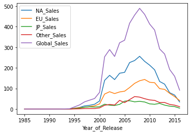
#년도별 각 지역의 판매량 합계
df[[x for x in df.columns if "Sales" in x] + ["Year_of_Release"]].groupby("Year_of_Release").sum()
| NA_Sales | EU_Sales | JP_Sales | Other_Sales | Global_Sales | |
|---|---|---|---|---|---|
| Year_of_Release | |||||
| 1985 | 0.00 | 0.03 | 0.00 | 0.01 | 0.03 |
| 1988 | 0.00 | 0.02 | 0.00 | 0.01 | 0.03 |
| 1992 | 0.02 | 0.00 | 0.00 | 0.00 | 0.03 |
| 1994 | 0.39 | 0.26 | 0.53 | 0.08 | 1.27 |
| 1996 | 7.91 | 6.88 | 4.06 | 1.24 | 20.10 |
| 1997 | 15.34 | 8.67 | 9.01 | 2.02 | 35.01 |
| 1998 | 18.13 | 12.13 | 10.81 | 2.14 | 43.18 |
| 1999 | 23.32 | 15.69 | 9.67 | 2.45 | 51.17 |
| 2000 | 39.34 | 25.20 | 11.27 | 5.49 | 81.24 |
| 2001 | 139.32 | 72.85 | 23.57 | 18.26 | 253.88 |
| 2002 | 163.76 | 84.03 | 18.61 | 22.30 | 288.84 |
| 2003 | 143.08 | 75.16 | 17.24 | 19.68 | 255.35 |
| 2004 | 173.88 | 83.01 | 22.74 | 42.14 | 321.78 |
| 2005 | 178.15 | 86.70 | 38.23 | 31.05 | 334.32 |
| 2006 | 225.69 | 104.53 | 40.43 | 45.90 | 416.72 |
| 2007 | 235.61 | 124.71 | 35.04 | 60.62 | 456.23 |
| 2008 | 256.25 | 137.31 | 37.42 | 57.89 | 489.12 |
| 2009 | 231.72 | 143.56 | 34.28 | 50.25 | 459.85 |
| 2010 | 213.24 | 130.13 | 25.19 | 44.24 | 412.96 |
| 2011 | 190.62 | 127.86 | 23.16 | 42.10 | 383.69 |
| 2012 | 133.94 | 99.08 | 27.36 | 31.57 | 291.93 |
| 2013 | 120.89 | 95.54 | 19.05 | 31.80 | 267.17 |
| 2014 | 79.38 | 76.42 | 14.02 | 22.58 | 192.43 |
| 2015 | 67.85 | 60.51 | 11.85 | 18.86 | 159.16 |
| 2016 | 34.52 | 41.03 | 4.34 | 11.59 | 91.56 |
# DataFrame plot
df[[x for x in df.columns if "Sales" in x] + ["Year_of_Release"]].groupby(
    "Year_of_Release"
).sum().plot();
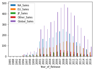
df[[x for x in df.columns if "Sales" in x] + ["Year_of_Release"]].groupby(
    "Year_of_Release"
).sum().plot(kind="bar");
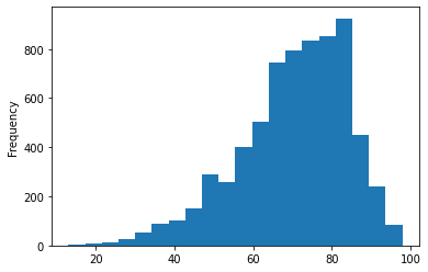
df['Critic_Score'].plot.hist(bins=20)
<matplotlib.axes._subplots.AxesSubplot at 0x7f08fba3a990>
import seaborn as sns
sns
seaborn: statistical data visualization
http://seaborn.pydata.org/
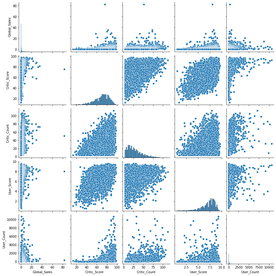
import seaborn as sns
sns.pairplot(
    df[["Global_Sales", "Critic_Score", "Critic_Count", "User_Score", "User_Count"]]
);
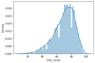
sns.distplot(df["Critic_Score"]);
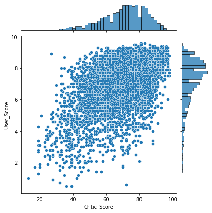
#jointplot
sns.jointplot(x="Critic_Score", y="User_Score", data=df, kind="scatter");
결론:
간단하게 pandas를 이용하여 데이터 분석을 해보았다. 알면 편하고 모르면 불편한 것이 라이브러리의 세계라고 생각한다.